Buckling in connections – stability as a separate limit state

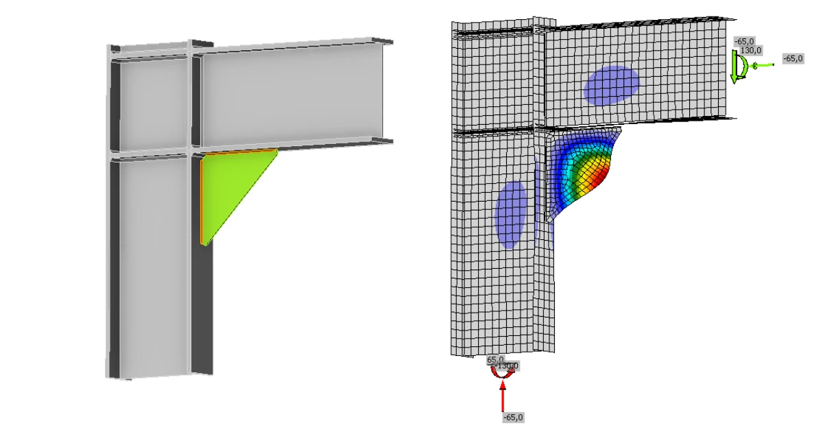
This article demonstrates how local stability in connection details can be systematically assessed using a practical workflow consisting of LBA, MNA, FE‑slenderness and subsequent reduction.

Why stability in connections is a separate limit state

A stress verification and a stability verification do not answer the same question. A stress verification essentially checks whether the material approaches its plastic limit. A stability verification, on the other hand, checks whether a member or a local region loses its load‑bearing capacity due to instability. A connection can therefore appear plausible from a stress perspective and still be locally critical with respect to stability.

Interpretation of EN 1993‑1‑5 for connection details

The rules of DIN EN 1993‑1‑5 originate mainly from comparatively large plate panels with well‑defined boundary conditions. Typical applications include web and flange panels, plate strips or other bridge design components where the structural behaviour can clearly be classified as plate buckling. 

However, a connection plate or node plate is not always exactly such a case. Boundary conditions, load paths and stress distributions in a connection are often more complex and locally more influenced than in the classical applications of the standard.

Therefore, the logic of EN 1993‑1‑5 should not be applied blindly to connection regions.
A prerequisite for its application is rather:

• that a truly plate‑like structural behaviour exists,
• that the in‑plane stresses govern the behaviour,
• and that the corresponding buckling mode is mechanically plausible as a plate buckling field.

If these prerequisites are not met, the structural behaviour should not be interpreted as purely plate‑like. In practice, the following areas are particularly susceptible to local stability effects:

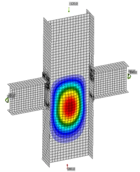
Column web under local compression

If a column web is loaded in transverse or local compression, the web panel may be prone to buckling even though the global structural system still exhibits significant reserve capacity.

$$\textsf{\textit{\footnotesize{Support beam under pressure}}}$$

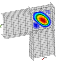
Shear panels

Shear panels may become stability‑relevant, particularly when high stress levels coincide with slender panel geometries.

$$\textsf{\textit{\footnotesize{Sliding panel in support}}}$$

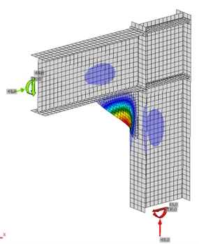
Stiffeners with free edges

Stiffeners may appear robust but can become locally unstable if free edges or column‑like buckling shapes dominate.

$$\textsf{\textit{\footnotesize{Triangular stiffness under pressure}}}$$

Strip‑like compression fields

With unfavourable restraints, a field may lose its plate‑like behaviour and respond more like a strip or column.

What Does the Critical Buckling Factor α_cr Represent?

The critical buckling factor α_cr is obtained from Linear Buckling Analysis (LBA). It represents the factor by which the applied load would need to be increased for the idealized elastic system to become unstable. α_cr is therefore useful for early identification of stability‑critical cases — but it is not a full verification.

Key points: 

• LBA uses idealized geometry,
• material plasticity is not considered,
• imperfections are not included.

Thus, α_cr is primarily a screening parameter.

What Does α_ult Represent?

The factor α_ult is obtained via a materially nonlinear analysis (MNA). It represents the proportional increase of the load until the defined plastic limit state is reached. In IDEA StatiCa, this corresponds to the 5% plastic strain criterion of the material model. α_ult therefore characterizes the plastic load reserve of the connection.

With specific regard to EN 1993‑1‑8, this aspect is of particular importance: ductility is a fundamental requirement to enable plastic redistribution within the joint and to avoid brittle failure modes. In this context, the MNA diagram provides a very useful additional piece of information. The x‑axis represents the strain in percent, while the y‑axis shows the load‑increase factor α_ult.

$$\textsf{\textit{\footnotesize{MNA diagram showing ductile behavior}}}$$

$$\textsf{\textit{\footnotesize{MNA diagram showing brittle behavior}}}$$

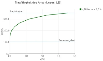
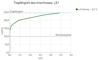
This allows for a clear assessment of whether plastic reserves in the plates are actually being mobilised:

• If plastic strains reach the order of approximately 5%, this is more indicative of ductile behaviour.
• If the resistance curve drops off early and only small plastic strains occur in the plates, this tends to indicate brittle behaviour.

However, the following remains important:

The MNA analysis alone does not constitute a stability check.

A pure MNA analysis does not include geometric imperfections and, by itself, does not answer the question of whether a detail is critical with respect to stability. For this reason, α_ult is not used in isolation in the procedure described here, but always in combination with α_cr.

Recommended Workflow in IDEA StatiCa

The following procedure is recommended for the practical assessment of local stability during installation.

Step 1 – Perform LBA

Determine α_cr and the corresponding eigenmode. Examine not only the numerical value but also the physical plausibility:

• Is the eigenmode mechanically meaningful?
• Which region becomes unstable?
• Is the behaviour plate‑like or rather strip/column‑like?

Step 2 – Perform MNA

Determine α_ult and identify available plastic reserve. Evaluate the load‑capacity curve to see whether plasticity is mobilized or whether the system fails earlier.

Step 3 – Determine FE‑based Slenderness

Compute slenderness:

$\lambda = \sqrt{\alpha_{\text{ult}} / \alpha_{\text{cr}}}$

This relates elastic instability tendency to the plastic reserve.

Step 4 – Choose Appropriate Reduction Approach

Depending on the behaviour:

• Plate‑like: reduction using ρ according to EN 1993‑1‑5
• Column‑like: reduction using χ according to EN 1993‑1‑1

Step 5 – Perform Verification

Only after reduction is the plastic reserve converted into a stability‑adjusted capacity.

Reduction according to EN 1993‑1‑5: Stocky, Intermediate, Slender

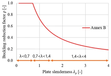
For plate‑like behaviour, stability reduction uses ρ from EN 1993‑1‑5 Annex B. The curve can be interpreted in three regions:

1. Stocky Range
$\lambda_p \le 0{,}7$

In this range, the following applies:
$\rho = 1$

No reduction is required. Stability effects are generally not governing, and the plastic resistance can be fully mobilised.

2. Transition Range
$0{,}7 < \lambda_p < 1{,}4$

In this range, the following applies:
$0{,}5 \lesssim \rho < 1$

Here, the reduction due to stability effects begins. The element is no longer stocky but not yet highly slender. Many practical cases fall within this range.

3. Highly Slender Range
$1{,}4 < \lambda_p < 4$

In this range, the following applies:
$0{,}5 \lesssim \rho \lesssim 0{,}2$

In this range, the reduction due to stability effects is already significant. The plastic reserve is considerably reduced, and instability governs the structural behaviour.

This three-part classification serves as a practical working definition. Annex B of EN 1993‑1‑5 provides the reduction function but does not explicitly define these three categories. However, for engineering assessment, this subdivision is very useful.

Plate‑like behaviour

A panel may be considered plate‑like if

• the structural behaviour is governed by in‑plane plate action,
• the boundary conditions can be described plausibly, and
• the buckling mode corresponds to a classical plate‑type buckling field.

In such cases, the reduction using ρ according to EN 1993‑1‑5 is appropriate.

Column‑like behaviour

A panel should rather be treated as column‑like if

• the buckling mode appears strip‑like,
• free edges dominate,
• the behaviour is no longer purely plate‑type, or
• a member‑like out‑of‑plane deformation pattern develops.

In such cases, a reduction using χ according to EN 1993‑1‑1 is often the more suitable choice.

The distinction between plate‑like and column‑like behaviour is, however, not always clear‑cut in practice. DIN EN 1993‑1‑5 also provides an interaction equation for such borderline cases. For connection details, this approach is generally too elaborate, especially when eigenmodes, boundary conditions, and local structural mechanisms can no longer be idealised in a reliable manner. In the method presented here, a deliberately simple and conservative procedure is adopted:

• If a clearly plate‑like buckling field is present, the reduction is performed with ρ according to EN 1993‑1‑5.
• As soon as column‑like behaviour or a buckling field with only two supported edges becomes relevant, we conservatively recommend a reduction with χ according to EN 1993‑1‑1 using buckling curve b.

This is not the mathematically most refined solution in every individual case, but it is robust and transparent for the practical assessment of local stability in connections.

Conservative Derivation of the Screening Thresholds

Screening values are not intended to replace the actual verification. They merely assist in determining whether a local buckling field is likely to be non‑critical or whether a more detailed assessment becomes necessary.
The derivation proceeds via the verification limit:

$\rho \cdot \alpha_{\text{ult}} / \gamma_{M1} \ge 1$

thus:

$\alpha_{\text{ult,min}} = \gamma_{M1} / \rho$

and then:

$\alpha_{\text{cr}} = \alpha_{\text{ult}} / \lambda^{2}$

For the conservative EN 1993‑1‑5 Annex B approach, at

$\lambda = 0.7$

we still have:

$\rho = 1$

Thus:

$\alpha_{\text{ult,min}} = 1.1 / 1 = 1.1$

$\alpha_{\text{cr}} = 1.1 / 0.49 = 2.245$

Therefore:

$\alpha_{\text{cr,min}} \approx 2.25$

For column‑like behaviour with reduction via χ according to EN 1993‑1‑1, buckling curve b:

$\alpha = 0.34$

at

$\bar{\lambda} = 0.7$

we obtain:

$\varphi = \tfrac{1}{2} \left[ 1 + \alpha (\bar{\lambda} - 0.2) + \bar{\lambda}^{2} \right]$

$\varphi = \tfrac{1}{2} \left[ 1 + 0.34(0.5) + 0.49 \right] = 0.83$

$\chi = \frac{1}{\varphi + \sqrt{\varphi^{2} - \bar{\lambda}^{2}}}$

$\chi \approx 0.784$

Then:

$\alpha_{\text{ult,min}} = 1.1 / 0.784 = 1.403$

$\alpha_{\text{cr}} = 1.403 / 0.49 = 2.864$

Therefore:

$\alpha_{\text{cr,min}} \approx 2.86$

For practical preliminary assessment, this is still rather tight. It is therefore useful to work with additional recommended conservative screening values.

Screening Thresholds

* For approximate illustration only. Not normative values, not a pass‑fail criterion, and not a substitute for the actual verification.

The following is important:

• the second column describes the derived minimum threshold,
• the third column describes the recommended conservative screening value.

This distinguishes between the computational lower limit and a robust preliminary assessment.

Example: Verification of a Shear Panel in a Column – Plate‑like Behaviour

In this example, a local buckling field is considered which can be mechanically classified as plate‑like.

$$\textsf{\textit{\footnotesize{Shear panel in a column}}}$$

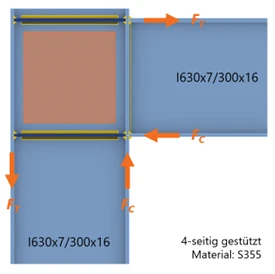
The LBA yields:

$\alpha_{\text{cr}} = 1.99$

Thus, the selected screening threshold is not reached. A more detailed verification is therefore required.
The subsequent MNA yields:

$\alpha_{\text{ult}} = 1.07$

From this, the FE slenderness is obtained:

$\lambda_p = \sqrt{\alpha_{\text{ult}} / \alpha_{\text{cr}}} = \sqrt{1.07 / 1.99} \approx 0.73$

The panel is thus only slightly outside the stocky range. Since the behaviour is classified as plate‑like, the reduction is performed using ρ according to EN 1993‑1‑5.
For the conservative approach, the following parameters are used:

$\lambda_{p0} = 0.70,\ \alpha_p = 0.34$

First,

$\varphi = \tfrac{1}{2} \left[ 1 + \alpha_p (\lambda_p - \lambda_{p0}) + \lambda_p^{2} \right]$

is calculated:

$\varphi = \tfrac{1}{2} \left[ 1 + 0.34(0.73 - 0.70) + 0.73^{2} \right] = 0.7716$

From this, the reduction factor follows:

$\rho = \frac{\varphi - \sqrt{\varphi^{2} - \lambda_p^{2}}}{\lambda_p^{2}} \approx 0.98$

The reduction is therefore very small. This corresponds to the classification that the panel lies only slightly outside the stocky range.

The verification is carried out using the reduced plastic resistance:

$\rho \cdot \alpha_{\text{ult}} / \gamma_{M1} \ge 1$

with

$\rho = 0.98,\ \alpha_{\text{ult}} = 1.07,\ \gamma_{M1} = 1.1$

Thus:

$\rho \cdot \alpha_{\text{ult}} / \gamma_{M1} \approx 0.95 < 1$

The verification is therefore not satisfied. The interesting conclusion of this example is:

• The screening threshold is missed only slightly.
• However, the stability reduction is very small at $\rho \approx 0.98$
• The actual issue is therefore not stability, but the limited plastic reserve.

Example: Verification of a Triangular Stiffener in Compression – Column‑like Behaviour

In this example, the buckling mode does not show a classical plate‑type field. The behaviour is partly column‑like, so the verification cannot sensibly be performed using plate logic alone.

$$\textsf{\textit{\footnotesize{Triangular stiffener in compression}}}$$

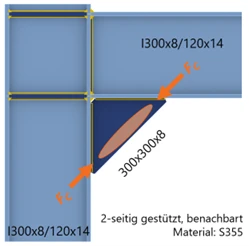
The LBA yields:

$\alpha_{\text{cr}} = 3.77$

Thus, the chosen screening threshold of 4.0 is not quite reached. This means: a more detailed verification is required.

The materially nonlinear analysis yields:

$\alpha_{\text{ult}} = 2.23$

Thus, a plastic reserve is present.

From α_ult​ and α_cr​, the slenderness is calculated:

$\lambda = \sqrt{\alpha_{\text{ult}} / \alpha_{\text{cr}}} = \sqrt{2.23 / 3.77} \approx 0.77$

Since the behaviour is column‑like, the reduction is not performed with ρ according to EN 1993‑1‑5, but with χ according to EN 1993‑1‑1, buckling curve b.

For buckling curve b, the imperfection factor according to EN 1993‑1‑1 is:

$\alpha = 0.34$

First,

$\varphi = \tfrac{1}{2} \left[ 1 + \alpha (\lambda - 0.2) + \lambda^{2} \right]$

is computed:

$\varphi = \tfrac{1}{2} \left[ 1 + 0.34(0.77 - 0.2) + 0.77^{2} \right] = 0.89335$

Then the reduction factor becomes:

$\chi = \frac{1}{\varphi + \sqrt{\varphi^{2} - \lambda^{2}}} \approx 0.74$

The verification is again performed using the reduced plastic resistance:

$\chi \cdot \alpha_{\text{ult}} / \gamma_{M1} \ge 1$

with

$\chi = 0.74,\ \alpha_{\text{ult}} = 2.23,\ \gamma_{M1} = 1.1$

Thus:

$\chi \cdot \alpha_{\text{ult}} / \gamma_{M1} \approx 1.50 > 1$

The verification is satisfied.

Geometrically, the case initially appears like a local panel. Mechanically, however, it must be treated rather as column‑like. Therefore, the reduction using χ is more robust here than a purely plate‑based assessment.

When is GMNIA the next step?

Not every case can be adequately represented using LBA, MNA, and subsequent reduction.
If details

• become very slender,
• are highly sensitive to imperfections, or
• involve more complex interactions,

then GMNIA is the next logical step.

With IDEA StatiCa Member, an appropriate tool is available for this. For typical connection plates, this is usually not the first step. For more complex or particularly critical cases, however, an extended GMNIA can be the correct continuation.

Conclusion

Local stability in connections should not be treated as a marginal topic. A pure stress check is insufficient.

It is not a single limit value that governs, but the methodological interplay between elastic instability, plastic reserve, and reduction.